Chapter 6: Climate Composites
Summary

Figure 6-1 The Climate Composites facilitates the analysis of a season among a group of non-consecutive years or compares the seasonal rainfall performance among two groups of years.
The Climate Composites tool (red box in Figure 6‑1) facilitates the analysis of a season among a group of years or compares the seasonal rainfall performance among two groups of years. For example: comparing the difference in rainfall conditions of the May–July (MJJ) season during El Niño and La Niña years in Central America. The Climate Composites tool calculates the seasonal average for a single group of years (EL Niño), the percent of average, as well as anomalies or standardized anomalies for one or two groups of years using an average baseline period.
6.1. Average
This function calculates the seasonal average for a group of years. El Niño (1982-83, 1986-87, 1987-88, 1991-92, 1997-1998, 2002-03, 2009-10, 2015-16) and La Niña (1988-89, 1998-99, 1999-00, 2007-08, 2010-11).
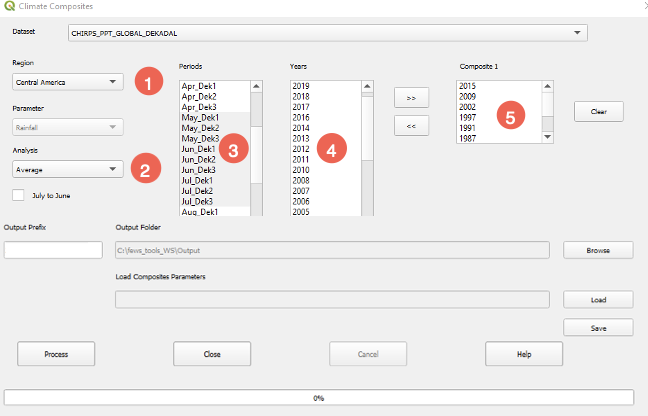
Figure 6-2 The Composites tool calculates the seasonal average from a group of years, among other functions.
To calculate the seasonal average for a group of years, follow the steps below:
Select the region of interest (Figure 6‑2 (1))
Select the method: In this case, select Average (Figure 6‑2 (2))
Select the season to be analyzed (Figure 6‑2 (3))
Select the years to be included for composite 1 (Figure 6‑2 (4))
Move the selected years to the composite 1 box by clicking the >> button (Figure 6‑2 (5)).
Click on Process. Figure 6-3 shows the results.
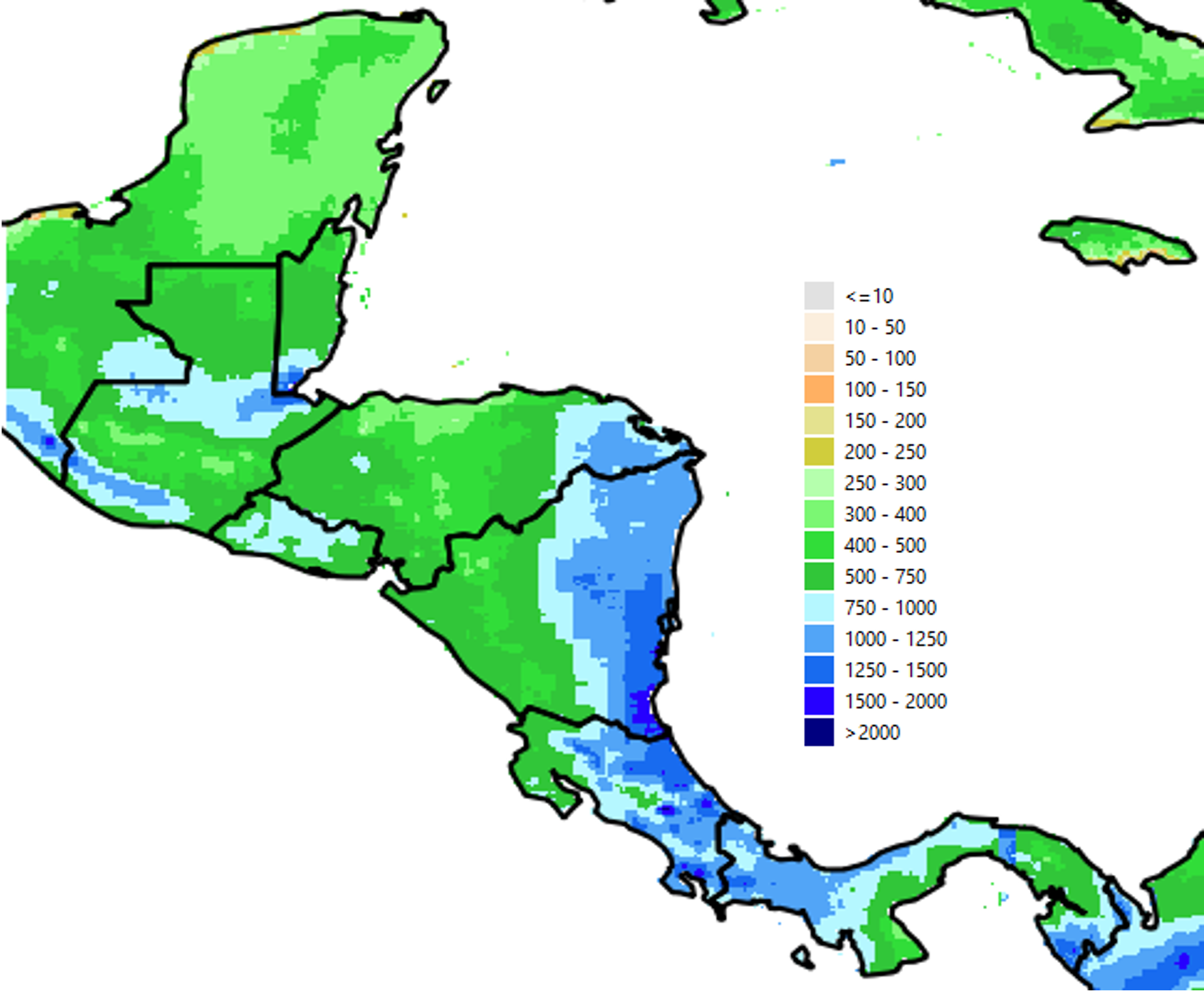
Figure 6-3 Average rainfall for El Niño years in Central America for the May - July season, composite 1.
6.2. Percent of Average (applies to composite 1 and composite 2):
The Percent of Average allows for the analysis of a single group of years or the comparison between two groups of years. Figure 6‑4 shows the input parameters: (1) La Niña years (composite 1), (2) El Niño years (composite 2), and (3) the Baseline, which indicates the period to be used to calculate the average.
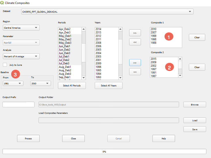
Figure 6-4 The composites function calculates the percent of average for a single group of years or compares two groups of years.
To calculate the percent of average for composite 1 (Equation 6.1):
Pctcomp1 = (averagecomp1 + (0.05*ltavg)+0.1 / averagebaseline + (0.05*ltavg)+0.1 ) * 100 (Equation 6.1)
If composite 2 is empty, the program saves pct_comp1 as the final output and displays the product.
If composite 2 is not empty, the program calculates the difference between the two composites as shown by Equation 6.2:
pctcomp = ((averagecomp1 - averagecomp2)+0.1 / averagebaseline+0.1) * 100 (Equation 6.2)
If (average_comp1 - average_comp2) = 0 or average_baseline = 0 then ((average_comp1 - average_comp2) / average_baseline) = 0, otherwise the results will come from Equation 6.2. In our example, Figure 6‑5 shows that rainfall is higher during La Niña years in most of the Pacific coast of Central America.
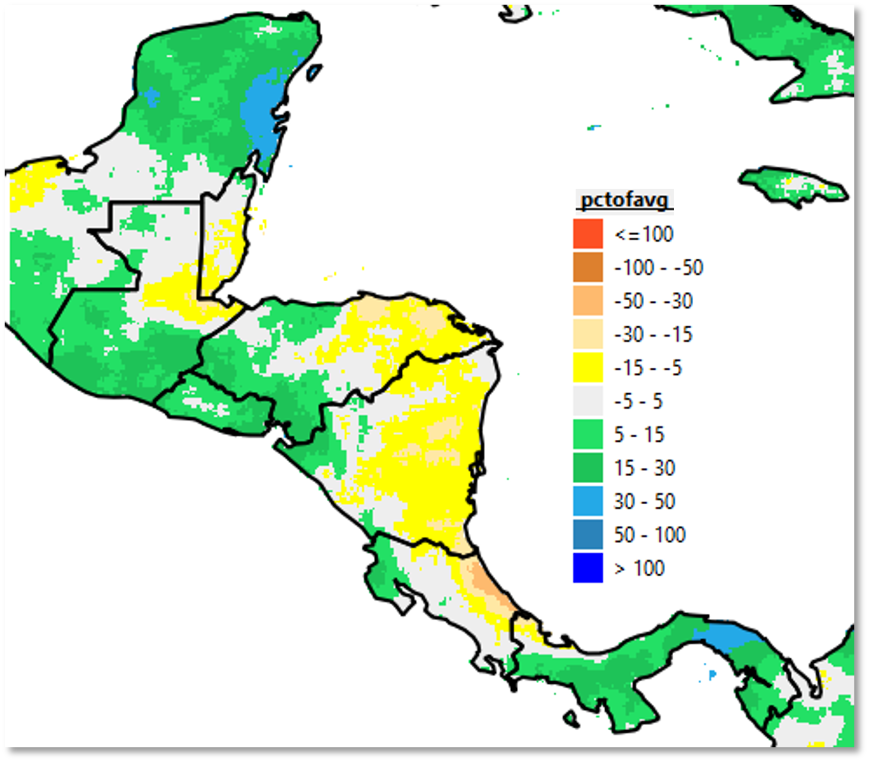
Figure 6-5 Percent of average for composites 1 (La Niña) and 2 (El Niño). In this example, the positive values indicate that precipitation during La Niña years is higher, on average, than during El Niño years.
6.3. Anomaly (applies to composite 1 and composite 2):
This analysis method calculates the average for each composite and the baseline; then, it calculates the anomaly for each composite (Equation 6.3).
anomcompN = averagecompN - averagebaseline (Equation 6.3)
If composite 2 is empty, the is saved as the final output and displayed on the QGIS canvas.
If composite 2 is not empty, the program calculates the difference between the anomalies of the two composites (Equation 6.4).
anomcomp = anomcomp1 - anomcomp2 (Equation 6.4)
Figure 6‑6 shows the results of the calculation of the anomalies for El Niño/La Niña example.
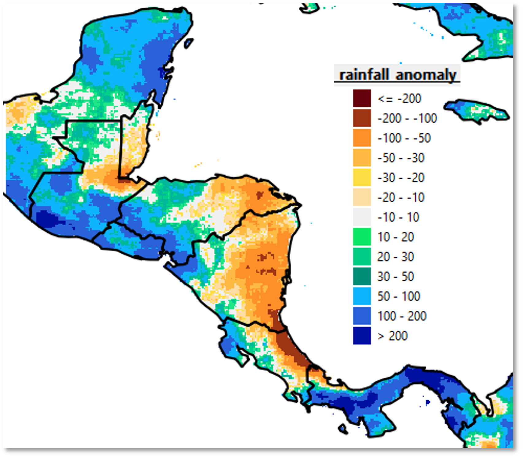
Figure 6-6 The positive anomalies show areas that were, on average, La Niña years have higher values than El Niño. The results are shown in mm. The default legend was modified based on the range of values.
6.4. Standardized Anomaly (applies to composite 1 and composite 2):
This analysis method calculates the difference anomaly, for the average seasonal precipitation, for each group of years and expresses it as a percent of the standard deviation. The function then subtracts the results of composite 2 from composite 1 and expresses it in terms of standard deviations away from the mean.
The method:
Validates if data exist for the selected years for composites 1 and 2, and baseline.
Calculates the standard deviation, including all the available years.
Calculates the average for the composites and baseline.
Calculates anomaly for each composite.
Calculates the standardized anomaly for each composite (Equation 6.5.)
stdanomcompN = ((averagecompN - averagebaseline) + 0.1 / stdevavailable years + 0.1) * 100 (Equation 6.5)
Where stdevavailable years is the standard deviation for all the years in the climate dataset for the selected period (e.g., period: May-July, composite1: El Niño years, baseline: 1981-2010, climate dataset: 1981-2017).
If composite 2 is empty, the function saves stdanomcomp1 as the final output and displays it in the Spatial Data Viewer.
If composite 2 is not empty, the function calculates the difference between the two composites as follows:
stdadnomcomp = stdanomcomp1 - stdanomcomp2 (Equation 6.6)
The results in Figure 6‑7 show the difference between composite 1 and 2 in terms of the standard deviation of the complete climate dataset. The areas in blue/purple show how much wetter on average El Niño years are than La Niña years, with the difference expressed in terms of standard deviations from the mean.
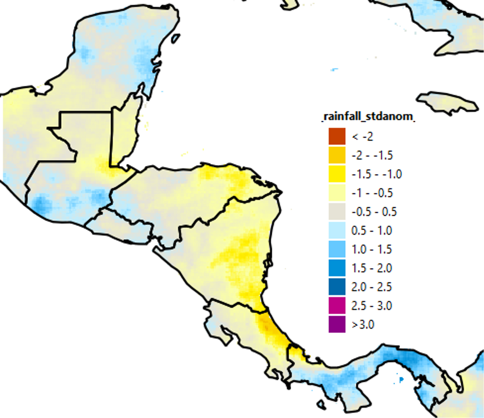
Figure 6-7 This function calculates standardized anomaly, which is the difference in anomaly of the average precipitation for a group of years (composite 1), expressed as a percent of the standard deviation. If composite 2 exists, the function calculates the difference between the two standardized anomalies.
NOTE: The raster values on the map shown in Figure 6‑7, are numbers with a scale factor of 100, since GeoCLIM does not work with decimals values. However, the legend shows the number of standard deviations from the mean.