Chapter 9: Background-Assisted Station Interpolation for Improved Climate Surfaces (BASIICS)
Summary

Figure 9-1 The Background-Assisted Station Interpolation for Improved Climate Surfaces (BASIICS) algorithm in GeoCLIM facilitates the improvement of climate variables by blending raster data with local stations, among other functions.
Satellite data provide useful information on climate variables (rainfall, temperature, and evapotranspiration) patterns. However, sometimes, satellite-estimated data contain biases and inaccuracies due to incorrect or limited ground data used during calibration. Some raster data also have a low spatial resolution, meaning the size of the pixel is too large for the area of interest. Such data could be improved by combining them with ground station information using the Background-Assisted Station Interpolation for Improved Climate Surfaces, (BASIICS) algorithm in GeoCLIM. See icon in red box in Figure 9‑1.
The BASIICS tool includes the following processes as shown in Figure 9‑2:
Blend climate raster/grids with stations (BASIICS)
Validate satellite data using ground station values
Interpolate stations only
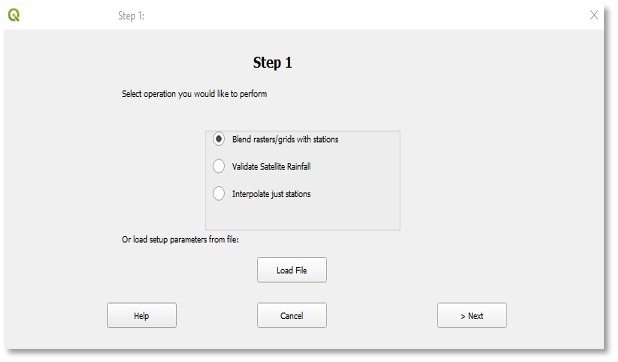
Figure 9-2 There are three options available in the BASIICS tool; (1) Blend stations and raster data, (2) Validate Satellite Rainfall and (3) Interpolate Just Stations.
The following three-step process is recommended to produce improved gridded datasets:
Use the download function or import the raster datasets to be improved, see chapter 2.
Use the Validate Satellite Rainfall to determine if the satellite and station data are correlated.
If they are correlated, blend the two datasets to produce improved rainfall estimates. Save the settings to a file so you could use it later to update the improved rainfall times series.
9.1. Validate satellite-based rainfall
The Validate Satellite Rainfall option allows you to evaluate grid/raster datasets (e.g., satellite-based rainfall estimates) using discrete points in space (e.g., rain gauges). The validation helps to determine if the two datasets are correlated to help in deciding if the blending option can be used with the two datasets to improve the raster using the point values by a blending process. The validation process first extracts values from a raster/grid at all locations where the point data have valid values (i.e., non-missing values. Missing values can be specified in the inputs). The results are: 1) A shapefile with the points that were included in the process. 2) A field of the interpolated values. 3) A .csv table that contain the station values, the corresponding grid value together with diagnostic information on the least-squares regression between the observed/in situ data value at the points being evaluated and the extracted grid values along with an R-squared output value. Once the correlation has been determined, then the raster and station data can be blended into an improved dataset.
To validate raster data, follow the three steps below:
9.1.1. Step 1: Select the BASIICS option
Click on the BASIICS icon from the main toolbar to open the dialog box (Step 1) (Figure 9‑1).
Select the ■ Validate Satellite Rainfall option. See Figure 9‑2.
Click on the > Next button to proceed to Step 2.
9.1.2. Step 2: Dataset and station parameters
Complete the form with raster and station data information. This form is made of 3 sections, (Figure 9‑3).
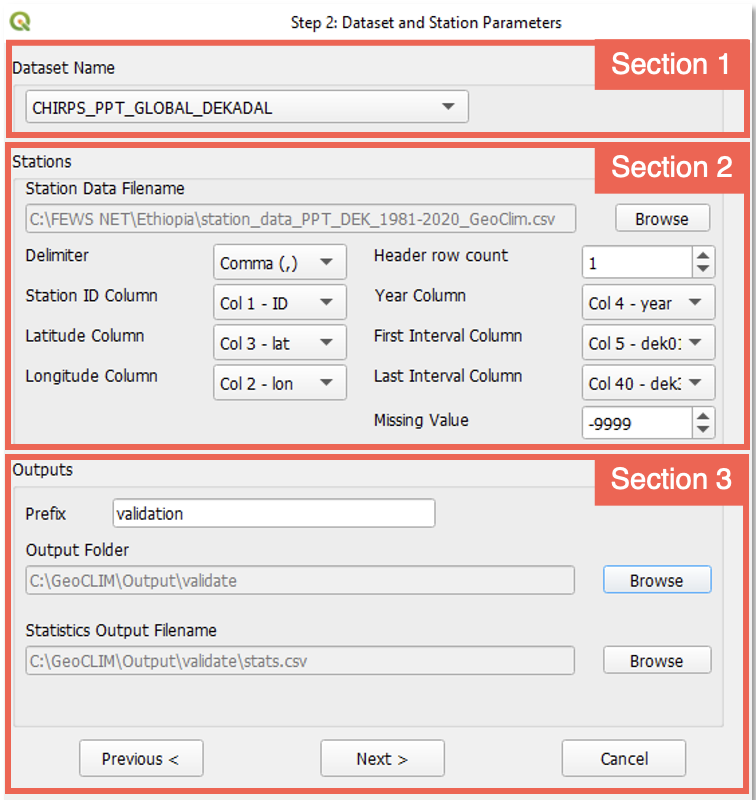
Figure 9-3 Step 2 allows you to enter the raster and station information for the validation.
9.1.2.1. Section 1: Grid Dataset Name
This section relates to the raster/grid input parameters. This process allows validation of climate datasets that have already been registered in GeoCLIM. To select the climate dataset to be validated, use the GeoCLIM dataset ˅ pulldown menu.
9.1.2.2. Section 2: Stations
This section relates to the station input parameters.
The tool assumes that all station data are in a single csv file. Browse to select the file that contains the station data. See an example in Figure 9‑4 of the file format. See the Data Management chapter for more information on the format of the table and other file types in GeoCLIM.
After selecting the station file, the tool identifies the header row and automatically completes the fields. Make any necessary changes to ensure that all field have the correct specification. When all the specifications are defined, move to section 3.
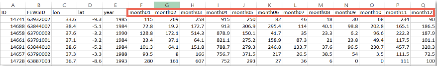
Figure 9-4 The CSV table with station data must contain a statin ID, lon, lat, year and a column for each pentad, dekad or month.
9.1.2.3. Section 3: Outputs
Specify the output prefix for all raster files created with the interpolation of the input stations.
Select the output folder.
Select the name for the statistics output file.
9.1.3. Step 3: Date parameters
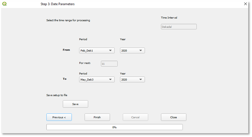
Figure 9-5 Step 3 allows you to select a period to validate and save the settings to use later.
Select the validation period as follows (see Figure 9‑5):
The time interval (e.g., month, dekad, or pentads) for the selected raster dataset is automatically displayed. Select the time range From and To of the raster data to validate. The time period and time interval are based on the selected climate dataset definition. In this example we are using dekads, see Figure 9‑5. And we are validating from (Feb dekad 01) to (May dekad 03), 2020.
Save the setup. At this step, you can save the validation settings so you could open it from step 1, edit and reuse it.
Click on the Finish button to run the process.
Outputs: The validation process creates the following outputs:
A shapefile, for each period, containing all the stations that were used in the process.
An interpolated field, for each period, using the IDW process (see Figure 9‑6a).
A scatterplot showing the satellite rainfall field values against the station values (Figure 96b).
A CSV file with columns containing the metadata for each station together with the station value, the corresponding raster value, and the at-station interpolated value. These at-station interpolated values are produced to improve comparability between the gridded/raster data and the station data. The CSV file includes statistics showing the correlation of the rainfall field and station data (Figure 9-6c).
These outputs provide the basis to decide if it is appropriate to blend the stations and the raster datasets.
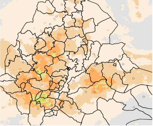
Figure 9-6a The validation process produces an interpolation field together with a shapefile containing all the points included.
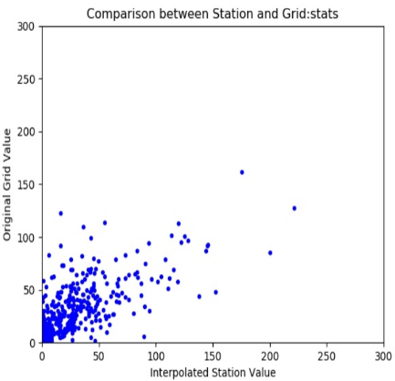
Figure 9-6b Scatterplot of interpolated station value on X and raster (CHIRPS) value on Y.
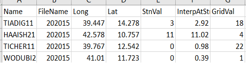
Figure 9-6c Text file that includes a list of the station value and its corresponding raster value for each date together with statistics describing their relationship.
9.2. Blend Rasters/Grids with Stations (BASIICS)
The blending algorithm is a methodology designed to combine station values such as rain gauges with raster/grid data, such as satellite-based estimates, to produce a more accurate gridded dataset. The algorithm combines the spatially discrete point data with spatially continuous grid data by interpolating the differences (ratios and anomalies) between the point and the grid value, where these two data are collocated. The blending is done using a modified Inverse Distance Weighting (IDW) method, which uses some concepts from the kriging method of interpolation, particularly simple and ordinary kriging. The technique is similar in principle to the SEDI technique that originates from the Southern African Development Community (SADC)/FAO Regional Remote Sensing Project, developed by Peter Hoefsloot.
9.2.1. Input Data for Blending
The program expects two types of data as described below:
A point dataset with values at discrete locations in space (example: rain gauges)
A grid dataset with values varying continuously over space (for example, a satellite-based rainfall estimate grid or a climatic average). For the algorithm to be used effectively, the two datasets need to be correlated.
9.2.2. The Process
Step 1. Extract values from the grid at all locations where the point data have valid values (missing values can be specified by the user). This produces a comparable dataset of grid values at the point locations that can be directly compared to the point values, see section 9.2 for validation.
Step 2. Multiplicative correction: A ratio is calculated between station and grid values; these ratios are interpolated using a modified IDW method, giving a maximum effective distance to each station. Once the maximum effective distance is reached, the interpolated layer takes the value of 1, (Figure 9‑7). The original rainfall layer is multiplied by the interpolated ratio layer. The pixels within a maximum effective distance of a station adjust the raster value based on the ratio, the pixels outside the influence of a station, that took the value of 1, take the value of the original raster layer.
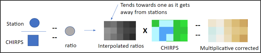
Figure 9-7 The first part of the blending process is a multiplicative correction based on the ratio between the station and the raster values.
Step 3. Additive correction: The anomaly between the station and the original raster is calculated at each point. The anomalies are interpolated using a modified IDW method, giving a maximum effective distance to each station. Once the maximum effective distance is reached, the interpolated layer takes the value of 0.
Step 4. The interpolated anomalies are added to the multiplicative corrected rainfall layer from step2 to obtain the Improved Rainfall Estimate (IRE), see Figure 9‑8.
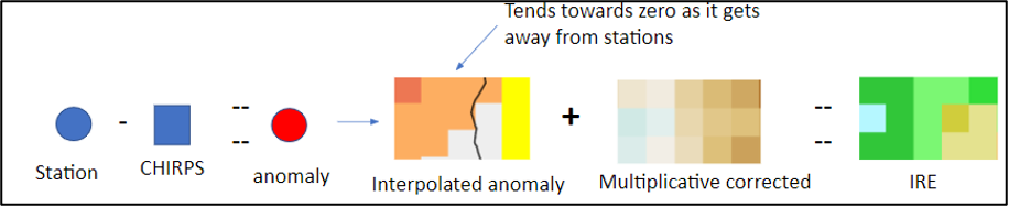
Figure 9-8 A second correction is done based on the anomalies between the station and the original raster values.
9.3. How to create improved rainfall estimates
9.3.1. Step 1: Select BASIICS option
Click on the BASIICS button from the main toolbar. See Figure 9‑1.
Select the ■ Blend rasters/grids with stations option. At this point you can click on the Load File button to load previously saved settings or click on the > Next button to start a new blending process. See Figure 9‑9.
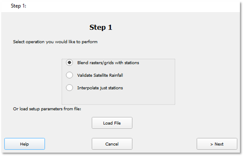
Figure 9-9 Select the Blend raster/grids with station option.
9.3.2. Step 2: Dataset and stations parameters
Complete the form with raster and station data information. This form is made of 5 sections (Figure 9-10).
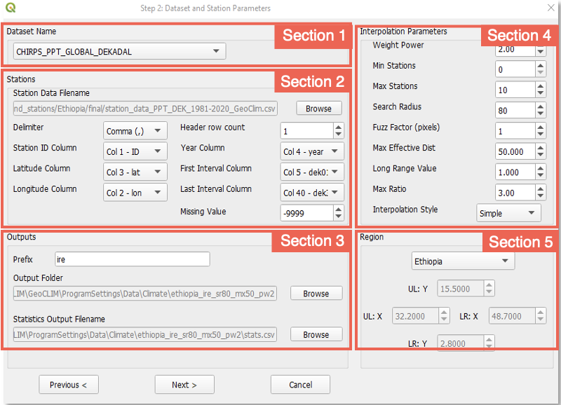
Figure 9-10 Step 3 of the blending process requires information about the raster data, the stations, the output location, the interpolation parameters, and the geographic domain.
9.3.2.1. Section 1: Grid dataset name
This section relates to the raster/grid input parameters. This process allows the improvement of climate datasets that have already been registered in GeoCLIM. To select the climate dataset to be used in the blending process, use the Dataset Name ˅ pulldown menu. In this example we are going to blend CHIRPS dekadal data with stations.
9.3.2.2. Section 2: Stations
This section relates to the station input parameters.
The tool assumes that all station data are in a single csv file. Browse to select the file which contains the station data. See an example in Figure 9‑11 of the file format. The order of the columns is not important, but must include the following:
A unique station identifier ID, in a single column.
A column with longitude in decimal degrees.
A column with latitude in decimal degrees.
A column with year value (yyyy).
A series of consecutive columns for the number of periods (72 for pentads, 36 for dekads, or 12 for months).
Any missing data should be completed with a single Missing Value, for example (-9999).

Figure 9-11 The CSV table with station data must contain a station ID, lon, lat, year and a column for each pentad, dekad or month.
Once you select the station file, the tool identifies the header row and automatically completes most of the fields. Make any necessary changes to ensure that all field have the correct specification.
9.3.2.3. Section 3: Outputs
In the third section, you can specify the output directory where to save the blended products. At this point, you have two options: (1) create a new dataset or (2) update an existing dataset.
Create a new dataset: This first option allows you to create a new dataset in the correct format so it works with the GeoCLIM functions; for example, you are blending, for the first time, your stations with the historical data of CHIRPS or CHIRP and want to create a new dataset from the results. To do this:
Provide a prefix for the output files.
Browse to the GeoCLIM data repository. For example: X:~\fews_tools_WS\ProgramSettings\Data\Climate\new_dataset where X:~ is the path to your GeoCLIM workspace.
The path on the Statistics Output Filename field changes automatically when you define the output directory.
Make sure to complete the fields in sections 4 and 5 before continuing. (See sections 4 and 5 for complete explanation of the parameters).
Click Next after completing all the fields.
A dialog box appears asking Do you want to create a new dataset from outputs?
Click on Yes.
Enter a new name with no spaces.
Select the data type.
Select the extent of the data. If your region is outside of Africa or Central America, please select global.
Click OK to move to Step 3.
Update an existing dataset: The second option is to add the latest record to an existing dataset. For example, you are blending the latest CHIRPS dekad with the stations and updating the time series you created previously.
In the Output folder field, browse to the existing directory X:~\fews_tools_WS\ProgramSettings\Data\Climate\existing_dataset where X:~ is the folder containing the workspace.
The path on the Statistics Output Filename field changes automatically when you specify the output directory.
Make sure to complete the fields in sections 4 and 5 before continuing. (See sections 4 and 5 for complete explanation of the parameters).
Click Next after completing all the fields.
A dialog box appears asking Do you want to create a new dataset from outputs?
Click on No to move to Step 3.
9.3.2.4. Section 4: The blending process - interpolation parameters
The program offers a set of options to adjust the parameters of the interpolation (Figure 9‑12).
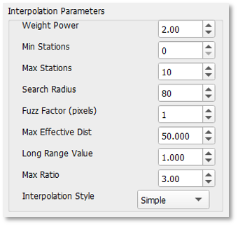
Figure 9-12 The blending process includes a series of parameters that you could modify.
Make sure you have a full understanding of the parameters before making any changes, otherwise, leave the default values. See a complete description of the parameters below.
Weight Power (WEIGHTPOWER): The power to which the inverse distance is raised in calculating the weight, indicating how fast the influence of the station decreases as the distance from the point increases. Figure 9‑13 shows an example of IDW with different powers.
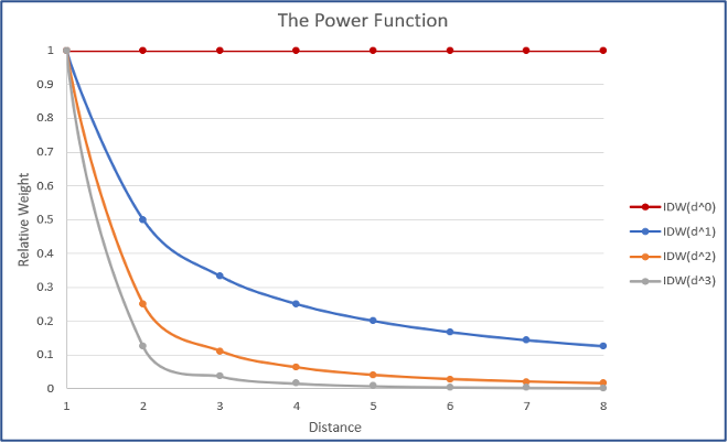
Figure 9-13 The power indicates how fast the relative weight decreases as distance increases.
Max Ratio (MAXRATIO): The maximum value allowed for the station/grid ratio. The program calculates the ratio between the station and grid values at each point location. The MaxRatio value limits this ratio to avoid “run-away” values in the process.
For example, assume that we are blending a rain gauge dataset with a satellite rainfall estimate. At station point A, the rainfall value is 10 mm, while the grid pixel value is 1 mm. Although the absolute difference between the two estimates is only 9 mm, the station/grid ratio is 10, or 1,000 percent. The ratio from all the points will be interpolated and then multiplied by the original grid. Assume that 50 km away from point A, the grid pixel had a value of 30 mm. This 30 mm will be multiplied by a value close to 10, depending on the surrounding ratios in the interpolation, and the resultant value may be close to 300 mm. This error can be limited by capping the ratio and instructing the program to cut off any ratios than a certain value (MAX RATIO). A cut-off ratio of 3 is used by default in the algorithm, meaning that any ratio greater than 3 is reset to 3 (in the example above, the ratio would be 3 instead of 10). However, this ratio can be set to any value by the user (a very large cut-off can be used; for example, 100,000) if you do not want to have the ratios capped.
Search Radius, Min Station, and Max Stations:
SEARCHRADIUS – the radius within which to search for points to be interpolated.
MINSTNS – minimum number of stations used in the interpolation.
MAXSTNS – maximum number of stations used in the interpolation.
The interpolation algorithm needs input values from the Min Stations (MINSTNS), the Max Stations (MAXSTNS), and the Search Radius (SEARCHRADIUS) fields for the pixel value estimation. At every pixel, the algorithm will search for the nearest stations within the SEARCHRADIUS from that pixel location and use the MINSTNS and the MAXSTNS to limit the number of stations to use during the interpolation.
For example, assume you defined the number of stations between 2 (MINSTNS) and 10 (MAXSTNS) to be used within a search radius of 200 km (SEARCHRADIUS). For this case, the algorithm will search for the nearest 10 stations within a radius of 200 km. If the number of stations found is less than 10 stations, for example, 7, then those 7 stations will be used. However, if the number of stations found is less than 2, then that location will have a missing value. Hence, for BASIICS, it is recommended to use an input value of 0 for MINSTNS, to produce a value everywhere in the output and avoid missing values.
Fuzz Factor (pixels) (FUZZFACTOR): The fuzz factor hides the location of the station by the number of pixels indicated in this field. A Fuzz Factor = 0 makes the value of the pixel near the station as close as possible to the station value.
Max Effective Distance (MAXEFFECTIVEDIST): This parameter is the maximum distance for which a station has influence over. This parameter only works with the Simple interpolation Style (idw_s, see the interpolation style section below). It is very important to consider the local characteristics of the region to choose a proper value for this parameter. We recommend you test different combination of values for the Max Effective distance and the search radius to avoid localized (bulls’ eye) effect around the station’s location.
Interpolation Style ˅ (INTERPOLATIONALGORITHM): The program provides two interpolation algorithms, Simple (idw_s) and Ordinary (idw_o) inverse distance weighting (IDW). In the ordinary IDW, the interpolation weights are dependent only on the surrounding stations. The Simple IDW method uses a background field to complete the interpolation. The background grid also contributes as a weight to the interpolation routine, and the relative weight of the background grid increases with increasing distance to surrounding stations.
9.3.2.5. Section 5 Region
Define Map Limits: Allows you to define the interpolation area (Figure 9-14). Make sure that the area is smaller or equal to the gridded dataset. This area can be defined by using the extent of an existing GeoCLIM Region or other spatial data (raster or vector). This option helps to speed up the interpolation process.
To run the blending process, follow the steps below:
Choose the region from the list.
Click on Next to move to step 3.
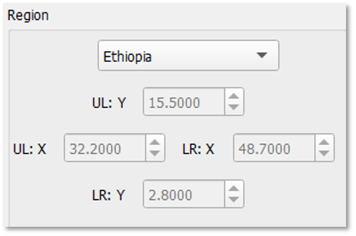
Figure 9-14 Select the region (basin, admin unit, etc.) for the new data.
9.3.3. Step 3: Date Parameters and Saving Settings
To save the date parameters and settings follow the steps below (Figure 9‑15):
The time interval (e.g., month, dekad, or pentads) for the selected raster dataset is automatically displayed.
Select the time range From and To of the data to blend. The time period and time interval are based on the selected climate dataset definition. In this example we are using dekads, see figure 9-17. And we are blending from Feb (dekad 01) to May (dekad 03) 2020.
Save the setup. At this step, you can save the blending settings so you could open it from step 1, edit and reuse it.
Click on the Finish button to run the process.
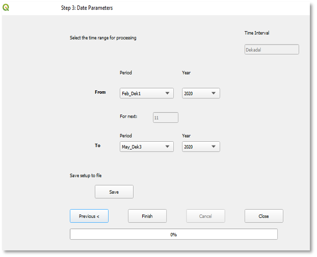
Figure 9-15 Step 3 allows you to define the time range for the blending process and you could also save the setting to use later.
9.4. Outputs: The blending process creates the following outputs:
A shapefile, for each period, containing all the stations that were used in the process.
The blended field, for each period. See Figure 9‑16a.
Three scatterplots showing the relationship of the original grid and the station values (Figure 9‑16b) for example.
A CSV file, (Figure 9‑16c) containing the metadata for each station together with the following columns:
Station value
Corresponding raster value
The BASIICS value at station location
Cross-validated BASIICS value. Indicates the BASIICS value at the station location without including that specific station in the process. This value responses to the question, what would be the value at this pixel if the station were not there.
Cross validated interpolation only. Pixel value of interpolation of stations only, without including the corresponding station.
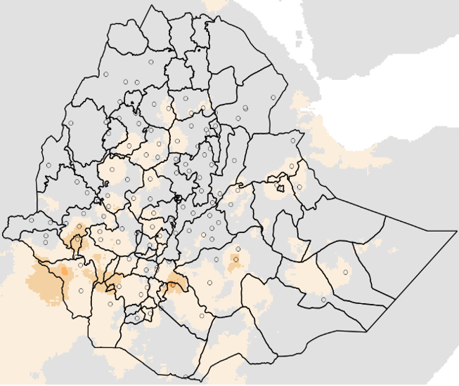
Figure 9-16a BASIICS field with participating stations.
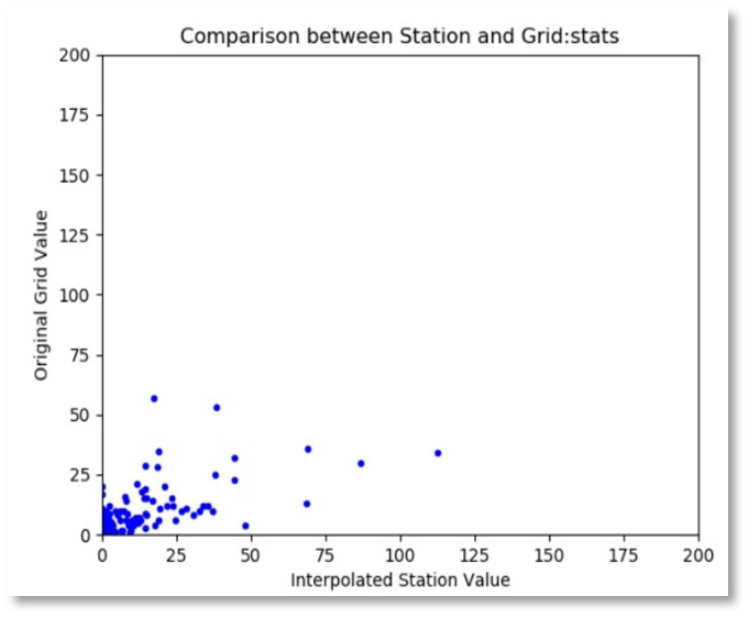
Figure 9-16b Comparison between station and raster values.
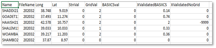
Figure 9-16c CSV table with information at station location.